SAS Programming for PK Time-Concentration Curve Using SGPLOT

Comparing with other software/tools for generating the graphs, SAS/Graph may be inferior. Programming to generate graphs using SAS/Graph languages can be time consuming and the quality of the graphs is usually not so great and not in publication quality. It is also not easy to output the graphs in the commonly used format. With SAS/Graph, we usually create the graph files in .cgm and then use a MS Word macro to load the .cgm files into MS Word file.

Now SAS has offered two new ways to generate the graphs: SASODS Graphics and SAS Stat Graphics. I had previously discussed SAS ODS Graphicswith template using Proc Lifetest to generate the Kaplan-Meier curve.

The procedure SGPLOT in SAS ODS Graphics can be used to generate high quality graph. With SGPLOT available, SAS/Graph procedure GPLOT become obsolete. The programs below illustrate the use of SGPLOT to generate the time-concentration curve for PK concentration data.

The graph generated from the programs is directly outputted in a .pdf file.

data pconc;

  input drug $ time concentration;

datalines;

Test  0   0

Test  1  32

Test  3 100

Test  6 140

Test  12 70

Test  24 25

Test  48  5

Test  72  1

Ref   0   0

Ref   1  40

Ref   3 105

Ref   6 135

Ref  12  80

Ref  24  28

Ref  48   7

Ref  72   0

;

options orientation=landscape nodate;

ods graphics / reset width=9in noborder;

    *width option defines the size of the graph. Noborder option remove  

     the border around the figure;

ods pdf file = "c:\temp\MySGPLOT.pdf"

 pdftoc = 0

 startpage = no

 style = printer

 dpi = 250;   

ods pdf nobookmarkgen;

title1 j=c "FIGURE #.#" ;

title2 j=c "MEAN PLASMA CONCENTRATION VS. TIME CURVES" ;

title3 j=c "BY TREATMENT" ;

title4 j=C "POPULATION:  PK" ;

footnote1 j=l "%upcase(PROGRAM: xxx.sas)                                                                                                                 (&sysdate &systime)";

run ;

proc sgplot data=pconc ;

    series x = time y = concentration

         /group=drug lineattrs = (thickness = 1 pattern=solid) markers;

    xaxis label = 'Time Post Study Drug Administration (hours)' 

         grid values = (0 to 80 by 5);

    yaxis label = 'Mean Concentration' grid values = (0 to 160 by 40); 

    keylegend / location=inside position=topright;

run;

ods pdf close;

References: 

• PROC SGPLOT over PROC GPLOT
• Using SAS® ODS Graphics
• ODS Statistical Graphics
• PK Plot with SGPLOT

Causality Assessment, Causality Categories for Reporting Adverse Events or Adverse Reactions

In clinical trials, safety reporting is a critical issue. This includes the reporting of safety information (adverse events or adverse reactions) from the investigational sites to the sponsor and then from sponsor to the regulatory agencies (FDA, EU) and distribution of the safety information to other investigational sites and IRBs. There have been many regulatory guidelines regarding the reporting of the safety information. However, none of the guidelines give clear instruction on how to categorize the causality for adverse events or adverse reactions.

In recent FDA’s guidance “Safety Reporting Requirements for INDs and BA/BE Studies”, it reiterates the concept of “reasonable possibility” for causality assessment, but does not provide the causality categories.

“Suspected adverse reaction means any adverse event for which there is a reasonable possibility that the drug caused the adverse event. For the purposes of IND safety reporting, ‘reasonable possibility’ means there is evidence to suggest a causal relationship between the drug and the adverse event. A suspected adverse reaction implies a lesser degree of certainty about causality than adverse reaction, which means any adverse event caused by a drug. Suspected adverse reactions are the subset of all adverse events for which there is a reasonable possibility that the drug caused the event. Inherent in this definition, and in the requirement to report suspected adverse reactions, is the need for the sponsor to evaluate the available evidence and make a judgment about the likelihood that the drug actually caused the adverse event. We consider the application of the reasonable possibility causality standard to be consistent with the discussion about causality in the International Conference on Harmonization (ICH) E2A Guideline (“ICH E2A guidance”)."

In FDA’s guidance “Good Pharmacovigilance Practices and Pharmacoepidemiologic Assessment”, they cited WHO, the Uppsala Monitoring Center, 2000, Safety Monitoring of Medicinal Product.

 “FDA does not recommend any specific categorization of causality, but the categories probable, possible, or unlikely have been used previously. If a causality assessment is undertaken, FDA suggests that the causal categories be specified and described in sufficient detail to understand the underlying logic in the classification.”

The regulatory guidance leaves the sponsor to decide what to be considered as ‘reasonable possibility’. The sponsor can design the data collection form (SAE form or adverse event case report form) using various categories for causality assessment/reporting.

For data collection purpose, what categories should be collected for causality assessment?

In ICH E2A CLINICAL SAFETY DATA MANAGEMENT: DEFINITIONS AND STANDARDS FOR EXPEDITED REPORTING”, there is a paragraph regarding the causality assessment and causality categories.  

“Many terms and scales are in use to describe the degree of causality (attributability) between a medicinal product and an event, such as certainly, definitely, probably, possibly or likely related or not related. Phrases such as "plausible relationship," "suspected causality," or "causal relationship cannot be ruled out" are also invoked to describe cause and effect. However, there is currently no standard international nomenclature. The expression "reasonable causal relationship" is meant to convey in general that there are facts (evidence) or arguments to suggest a causal relationship. “

In FDA guidance for reviewer “Conducting a Clinical Safety Review of a New Product Application and Preparing a Report on the Review, the following categories are referenced:

Causality assessment by investigator (definitely; probably; possibly; unlikely related)

In ICH E2B “MAINTENANCE OF THE ICH GUIDELINE ON CLINICAL SAFETY DATA MANAGEMENT: DATA ELEMENTS FOR TRANSMISSION OF INDIVIDUAL CASE SAFETY REPORTS “, the following causality categories are referenced in the examples provided in the guidelines. It turns out that these categories seem to be the most commonly used in practice.

The CDISC, CDASH considered causality assessment (relationship to study treatment) as a sponsored defined field. However, it recommends the categories listed in ICH E2B example:

“Sponsored-defined terminology will be used to indicate the relationship between the AE and the study treatment (e.g. ICH E2B examples: Not Related, Unlikely Related, Possibly Related, Related). “

EU regulations regarding the safety report are generally consistent with the ICH guidance (specifically ICH EB2) and do not provide any specific guidance on specific causality categories to use.

EMA Guideline on Good Pharmacovigilance Practice (GPV) recommends the following:

Different methods may be applied for assessing the causal role of a medicinal product on the reported adverse event (e.g. WHO-UMC system for standardised case causality assessment). In this situation, the levels of causality, which correspond to a reasonable possibility of causal relationship, should be established in advance in order to determine when an adverse event is considered as an adverse reaction.

Some sponsors used the causality categories from WHO 2000 Safety Monitoring of Medicinal Product that used the following categories. Definitely Probably Possibly Unlikely Conditional Related Related Related Related. For example, A FDA communication with Cangene Corporation indicated the following AE causality categories are used: Definitely related, Probably related, Possibly related, Unlikely related, and Conditional. This is the same as the above-mentioned WHO-UMC system for standardised case causality assessment.

CAUSALITY CATEGORIES

The causality categories described by the Uppsala Monitoring Centre are as follows. However, the following categories may be modified in the practical use. 

1. Certain: a clinical event, including laboratory test abnormality, occurring in a plausible time relationship to drug administration, and which cannot be explained by concurrent disease or other drugs or chemicals. The response to withdrawal of the drug (dechallenge) should be clinically plausible. The event must be definitive pharmacologically or phenomenologically, using a satisfactory rechallenge procedure if necessary.
2. Probable/Likely: a clinical event, including laboratory test abnormality, with a reasonable time sequence to administration of the drug, unlikely to be attributed to concurrent disease or other drugs or chemicals, and which follows a clinically reasonable response on withdrawal (dechallenge). Rechallenge information is not required to fulfil this definition.
3. Possible: a clinical event, including laboratory test abnormality, with a reasonable time sequence to administrations of the drug, but which could also be explained by concurrent disease or other drugs or chemicals. Information on drug withdrawal may be lacking or unclear.
4. Unlikely: a clinical event, including laboratory test abnormality, with a temporal relationship to drug administration which makes a causal relationship improbable, and in which other drugs, chemicals or underlying disease provide plausible explanations.
5. Conditional/Unclassified: a clinical event, including laboratory test abnormality, reported as an adverse reaction, about which more data is essential for a proper assessment, or the additional data is under examination.
6. Unassessable/Unclassifiable: a report suggesting an adverse reaction which cannot be judged because information is insufficient or contradictory, and which cannot be supplemented or verified.

Some sponsors may use the following categories and definitions for AE causality. For example, an NDA review memo from FDA indicated that the sponsor used the following causality categories: probable, possible, unlikely and not assessable. The instructions for the AE causality assessment are explained below:

Relationship to Investigational ProductThe assessment of the relationship of an adverse event to the administration of study drug (none, unlikely (remote), possible, probable, not assessable) is a clinical decision based on all available information at the time of the completion of the case report form.
None – includes: (1) the existence of a clear alternative explanation (e.g. mechanical bleeding at surgical site); or (2) non-plausibility (e.g., the patient is struck by an automobile at least where there is no indication that the drug caused disorientation that may have led to the event; cancer developing a few days after drug administration).
Unlikely (remote) – a clinical event, including lab abnormality, with an improbable time sequence to drug administration and in which other drugs, chemicals or underlying disease provide plausible explanation.
Possible – a clinical event including lab abnormality, with a reasonable time sequence to administration of the drug, which could also be explained by concurrent disease* or other drugs or chemicals.  Information on drug withdrawal may be lacking or unclear.
Probable – a clinical event including lab abnormality, with a reasonable time sequence to administration of the drug, unlikely to be attributed to concurrent disease* or other drugs or chemicals, and which follows a clinically reasonable response on withdrawal (dechallenge).
Not assessable – a report of an AE which cannot be judged because information is insufficient or contradictory, and which cannot be supplemented or verified.

Table below summarized various causality categories:

ICH E2B	Not Related, Unlikely Related, Possibly Related, Related)
CDISC	Not Related, Unlikely Related, Possibly Related, Related).
WHO	Certain, Probable/Likely, Possible, Unlikely, Conditional/Unclassified
Other options	None, Unlikely, Possible, Probable, Not assessable

Due to the fact that there is no clear regulatory guidance on the use of the causality categories, different sponsors could use different causality categories. The consequence is that the so-called drug–related adverse events (or the new term adverse drug reactions) can not be directly compared across the studies by different sponsors. The biases can arise if we attempt to compare the results from different studies conducted by different sponsors where the different causality categories are used. 

Submit the Clinical Trial Datasets to FDA: Using the right .xpt file format

When we submit the clinical trial datasets to FDA, we need to convert the datasets in original format (.sas7bdat) to .xpt format. There are two ways to convert the SAS datasets to .xpt format. However, only the .xpt format generated with Proc Copy can be accepted by FDA.

In FDA’s Study Data Specifications, section 2 (dataset specifications) is very specific about the data format that FDA will accept. It emphasized that "SAS transport file processed by the CPORT SAS PROC cannot be processed or achieved by the FDA"

2.1 File Format

SAS XPORT Transport File format

SAS XPORT transport file format, also called Version 5 SAS transport format, is an open format published by the SAS Institute. The description of this SAS transport file format is in the public domain. Data can be translated to and from this SAS transport format to other commonly used formats without the use of programs from SAS Institute or any specific vendor.
Version

In SAS, SAS XPORT transport files are created by PROC XCOPY in Version 5 of SAS software and by the XPORT SAS PROC in Version 6 and higher of SAS Software. SAS Transport files processed by the CPORT SAS PROC cannot be processed or archived by the FDA.

Sponsors can find the record layout for SAS XPORT transport files through SAS technical support technical document TS-140. This document and additional information about the SAS Transport file layout can be found on the SAS World Wide Web page at http://www.sas.com/fda-esub.

Transformation of Datasets

SAS XPORT transport files can be converted to various other formats using commercially available off the shelf software.

SAS Transport File Extension

All SAS XPORT transport files should use .xpt as the file extension.

Compression of SAS Transport Files

SAS transport files should not be compressed. There should be one dataset per transport file.

On SAS’s FDA Standards for Electronic Submissions, the differences between two different .xpt file formats are explained in Question & Answer format:

Q. There are two SAS transport file formats. Which one is the FDA prepared to use?

A. FDA can accept data in the SAS XPORT Transport Format that is processed by the XPORT engine in Version 6 of SAS software and later, and by PROC XCOPY in Version 5. 

Q. What are the two SAS transport formats?

A. The XPORT Transport Format selected by the FDA, and the CPORT Transport Format. Both XPORT and CPORT are established mechanisms for data exchange that are well tested and well documented. They are not new or at-risk technology. The XPORT Transport Format is supported on all platforms and releases of the SAS System (it is machine and release independent) from Version 5 on. The CPORT Transport Format was invented in Version 6 and is supported from Version 6 on.

Q. Why did FDA choose the XPORT Transport Format over CPORT Transport Format?

A. XPORT is an open format, while CPORT is a proprietary format.

Q. What do you mean, the XPORT format is "open?"

A. Specifications for the XPORT transport format are in the public domain. Data can be translated to and from the XPORT transport format to other commonly used formats without the use of programs from SAS Institute or any specific vendor.

Q. Why does FDA want an open format?

A. By US law, the FDA must remain "vendor neutral." The FDA cannot endorse or require use of any specific vendor's product.

Q. What is the XPORT transport format, generally?

A. It is a text file, with record length = 80 columns. It looks and feels so much like a text file that it is a good idea to avoid using ".txt" as a file name extension so that the operating system won't treat it as a text file.

When submitting the SAS datasets to FDA, we need to be sure that the .xpt files are generated using PROC COPY. After the .xpt files are generated, we should test if the files can be opened using JMP and SAS Viewer. If the .xpt files are generated correctly, they should be automatically opened if we click the file names.
According to SAS document on PROC COPY, it is very easy to use PROC COPY to create .xpt file.

libname source 'SAS-library-on-sending-host';

                     /*indicating where the original SAS data sets (in .sas7bdat format) are*/

libname xptout xport 'filename-on-sending-host'; 

                      /*indicating where the .xpt files to be stored */
proc copy in=source out=xptout memtype=data;
run;

Alternatively, .xpt files can be created using PROC CPORT. However, .xpt files created by PROC CPORT can not be opened with JMP and can not be opened in SAS Viewer. .xpt file created by PROC CPORT must be opened and retrieved by using PROC CIMPORT.

Since FDA will only accept the .xpt files generated using PROC COPY, I see no reason to use PROC CPORT or PROC CIMPORT.

Placebo Mean Imputation (PMI)

A while ago, I discussed several simple imputation methods in LOCF, BOCF, WOCF, and MVTF. Recently, I noticed another simple imputation method Placebo Mean Imputation (PMI). This simple imputation method of PMI seems to be used Only for the purpose of sensitivity analyses, not for the primary analysis. It is also true that this approach is mainly used in certain therapeutic areas such as analgesic drug (pain medication) and anti-bacterial drug.  

 

In FDA's Clinical Review document for a chronic pain medication in 2011,  the Placebo mean imputation is described:

 "Placebo mean imputation (PMI): the missing pain measurements for each day after discontinuation were replaced by the mean of all available pain intensity scores for all placebo-treated patients who completed treatment. Therefore if a patient discontinued treatment or recorded their last pain score at Week 8 of the Maintenance Period, the pain intensity score at Week 12 was imputed using the Week 12 mean pain intensity score for all placebo-treated patients who completed treatment. Also a placebo missing pain score at some time-point was imputed by the observed placebo group mean pain intensity at the same time-point"

In FDA's Statistical Review for the same indication, FDA statistician assessed that PMI is not an appropriate approach

"Since the estimated treatment effect is only influenced by the data from patients completing the study, the PMI method is similar to an analysis of completers. Analyzing completers is
problematic since the outcome of patients completing the study may not represent the outcome of patients not completing the study. In the placebo group, patients completing the study are likely to be the less severely afflicted patients; while in the NUCYNTA group, patients completing the study are likely to be the more severely afflicted patients. As a result, the PMI method assigned good scores from the placebo completers to patients dropping out due to adverse events in the treatment group. Based on these reasons, I conclude that the PMI method is not appropriate."

In a briefing document for FDA anti-infective drug advisory committee meeting for a cystic fibrosis drug in 2012, PMI approach was used by FDA statistical reviewer:

“…In this sensitivity analysis, missing values were imputed using the placebo group mean of -0.57% (i.e. the minimum of 0 and the least favorable group mean) as performed in the Reviewer’s primary analysis and other Reviewer analyses.”

The use of these simple imputation approaches is mainly driven by the perception that these approaches provide conservative estimate of the treatment effect (people have shown that this is not always true). This fits into the Intention-to-treat principle to be conservative in estimating the treatment effect in superiority studies. While it is ok to perform the sensitivity analyses using various simple imputation approaches such as LOCF, BOCF, WOCF, and PMI, these imputation methods should not be used as the primary analysis. 

Further Reading: 

• Gual et al (2013) A randomised, double-blind, placebo-controlled, efficacy study of nalmefene, as-needed use, in patients with alcohol dependence 
• Carpenter and Kenward (2007) Missing data in randomised controlled trials — a practical guide
• The National Academy Press (2010) The Prevention and Treatment of Missing Data in Clinical Trials

Replies to Inquiries to FDA on Good Clinical Practice

Good Clinical Practice (GCP) is the law of conducting the clinical trials. Sometimes, interpreting the law is challenging, the same is true in interpreting the GCP and other regulatory guidelines. FDA has set up an Office of Good Clinical Practice and provided  Good Clinical Practice Contacts for helping interpreting the GCP and answering the GCP related questions.

Recently, I just found that the FDA has an email address for questions and answers regarding GCP questions. The original questions along with FDA's responses are posted on the web. While FDA's responses may not directly address the original questions being asked, Replies to Inquiries to FDA on Good Clinical Practice is still a great resource.

•  Replies to Inquiries to FDA on Good Clinical Practice

Monitoring the double-blind study: unblinded pharmacist, unblinded monitor, and drug kit

In many clinical trials with biological products, the investigational products usually need to be reconstituted before the use. If the study is a double-blind study, the reconstitution of the investigational products can not be performed by the investigator in order for the investigator to remain blinded to the treatment assignment.

There are two ways to tackle this issue.

1. Using a third party (unblinded pharmacist).

With this option, the unblinded pharmacist at the investigational site will be the only person who knows the treatment assignment. The unblinded pharmacist will obtain the randomization number and treatment assignment information from the randomization envelope (manual process) or from IRT (interactive response technology including IVR or IWR) system. The unblinded pharmacist will then prepare and reconstitute the study drug, and then give to the investigator for administration.

The unblinded pharmacist must not communicate with the investigator about the subject treatment assignment.

The unblinded pharmacist must maintain the records for drug accountability for auditing and inspections.

With this option, the study team will need to include an unblinded CRA (clinical research associate) for the purpose of checking the drug accountability. In other words, there should be separate roles for two type of clinical monitors:

• Blinded Monitor: A monitor designated to perform site monitoring activities except for pharmacy, drug accountability, and reconciliation of the blinded investigational products.
• Unblinded Monitor: A monitor designated to perform the site monitoring activities for pharmacy, drug accountability, and reconciliation of the blinded investigational products.

 Some of the references for this approach:

• Unblinded Monitoring Programs: Design and Education
• Unblinded Monitoring in HCV Trials
• Integrated monitoring: Setting new standards for the next decade of clinical trial practice

2. Using the blinded drug kit for the investigational product  

With this approach, in addition to the randomization schedule (containing the  randomization number and the treatment assignment), additional list of drug kit numbers (and the linked batch or lot number corresponding to the investigational products) will be generated. Through the packaging, the label for the investigational product kit will contain only the kit number. Investigators can dispense or administer the investigational products to the patients based on the kit number without knowing the actual contents and the treatment assignments.

There is no need to have separate roles for site monitoring (ie, unblinded monitor and blinded monitor). The same monitor can cover the study activities and the pharmacy/drug accountability.

This approach can also be used for pills (non-biological products). It is especially useful when the investigational products are dispensed to the patients for their self-administration.  

A couple of examples for using this approach are listed below:

• Tenecteplase (TNK) study in AMI

“Randomization was to be blocked by study site, based on a SAS-generated code. Treatment assignment was made through a call to a centralized interactive voice response system for a drug kit number. Subjects were considered randomized upon verbal assignment of kit number.”

• A Randomized, Double-Blind, Placebo-Controlled Study of Guanfacine Extended Release in Children and Adolescents With Attention-Deficit/Hyperactivity Disorder

“Patients were randomly assigned to 1 of 3 groups of GXR treatment (2, 3, or 4 mg/day) or placebo, in a 1:1:1:1 ratio. Matching GXR and placebo tablets were provided to patients in the form of weekly prepackaged individual study drug kits, identical in appearance, according to the randomization schedule. Every morning during the double-blind treatment period, patients took a total of 4 tablets, without regard to meals. Patients who completed the screening and washout periods were assigned to the treatment group of the next available drug kit in ascending order of the drug kit number (or randomization number), which was recorded on the case report form.”

Science or Just for Fun? - Correlation between Chocolate Consumption and Winning Nobel Prize

 The New England Journal of Medicine is a very prestigious medical journal with very high impact factor. I am surprised to read an article by Dr Messerli to claim that the chocolate consumption is correlated to winning the Nobel Laureates. See “Chocolate Consumption, Cognitive Function,and Nobel Laureates” at NEJM 367;16 1562-1564.

I hope that the paper was published just for fun, not for serious discussion of the science.

Nothing is wrong about the statistical calculation. The p-value for correlation coefficient is indeed statistically significant. However, this superficial correlation ignores many confounding factors behind this correlation. I guess that it will be embarrassing to find out that even though there is a correlation between the chocolate consumption on national level and the number of Nobel Laureates, the Novel Laureates are those who consumed little or no chocolate.

In my first college lesson about the correlation, the teacher told me that before calculating the correlation coefficient, make sure that we were comparing two things that are related. If we try to claim there is a correlation between the growth of a tree and a growth of a baby, we will certainly be able to establish the correlation, but so what?

An excerpt from J. A. Paulos,Beyond Numeracy gives some examples that the wrong correlations are assumed.

“Children with bigger feet spell better. In areas of the South those counties with higher divorce rates generally have lower death rates. Nations that add fluoride to their water have a higher cancer rate than those that don't. Should we be stretching our children's feet? Are more hedonist articles in Penthouse and Cosmopolitan on the way? Is fluoridation a plot?
……
The odd results above are easily explained in this way. Children with bigger feet spell better because they're older, their greater age bringing about bigger feet and, not quite so certainly, better spelling. Age is a factor in the next example as well since those couples who are older are less likely to divorce and more likely to die than are those from counties with younger demographic profiles. And those nations that add fluoride to their water are generally wealthier and more health-conscious, and thus a greater percentage of their citizens live long enough to develop cancer, which is, to a large extent, a disease of old age.”

Unfortunately, nowadays, many articles in medical journals consciously or unconsciously presents the correlations between two things without further considering the confounding factors or the basis for the correlations. This is why we often see that a conclusion from one study is later totally reversed by the results from the another study.

Fields Arranged by Purity - A Cartoon

See the explanation for this cartoon, please visit: explainxkcd.com

‘As treated’ versus ‘As randomized’ analysis

When we design a non-inferiority trial to support the product registration, the regulatory agencies may suggest the statistical analysis using ‘as treated’ population. In FDA’s Guidance for Industry Non-Inferiority Clinical Trials, it suggested the ‘as-treated’ analysis for primary efficacy endpoint:

“Intent-to-treat (ITT) analyses in superiority trials are nonetheless preferred because they protect against the kinds of bias that might be associated with early departure from the study. In non-inferiority trials, many kinds of problems fatal to a superiority trial, such as non-adherence, misclassification of the primary endpoint, or measurement problems more generally (i.e., “noise”), or many dropouts who must be assessed as part of the treated group, can bias toward no treatment difference (success) and undermine the validity of the trial, creating apparent non-inferiority where it did not really exist. Although an “as-treated” analysis is therefore often suggested as the primary analysis for NI studies, there are also significant concerns with the possibility of informative censoring in an as-treated analysis. It is therefore important to conduct both ITT and as-treated analyses in NI studies. Differences in results using the two analyses will need close examination.”

The term “as treated” means that when we do analysis/summaries, the treatment assignment is based on the actual treatment the patients receive, not the treatment the patients are supposed to receive. The concept of “as treated” should be explained in comparison with “as randomized” – a key component for the concept of “Intention-to-Treat” principle.

Typically, ‘Intention-to-Treat’ population can be simply defined as all patients who are randomized. However, the formal definition of the “Intention-to-Treat” population contains several other concepts:

The formal definition of the "Intention to Treat" is usually referred to the one suggested by Fisher, LD et al. in “Intention to treat in clinical trials in Statistical Issues in Drug Research and Development. Edited by Peace KE (1990)”. Intention to Treat population “Includes all randomized patients in the groups to which they were randomly assigned, regardless of their adherence with the entry criteria, regardless of the treatment they actually received, and regardless of subsequent withdrawal from treatment or deviation from the protocol”.

In other words, ITT analysis includes every subject who is randomized according to randomized treatment assignment. It ignores noncompliance, protocol deviations, withdrawal, and anything that happens after randomization. ITT analysis is usually described as “once randomized, always analyzed”. ITT analysis is referred as ‘as randomized’ - the opposite of the term ‘as treated’.

In majority of cases, if all randomized subjects receive their allocated treatments and if there is no randomization error, the ‘as treated’ analysis will be the same as 'as randomized' analysis.

If some randomized subjects do not receive the randomly alloccated treatment and if there are randomization errors, ‘as treated’ population will be different from ITT population or 'as randomized' population.

The example below can be used to illustrate the difference between the ‘as treated’ and ‘as randomized’. This is an open label, randomized study to compare the treatment effect of r-ProUK (intra-artery prourokinase + heparin) with control (heparin alone) on acute ischemia stroke - PROACT II Study. Eligible subjects were randomized to r-proUK or Control in 2:1 ratio. 180 subjects were randomized (121 subjects to r-proUK group and 59 to Control group). The problem was that in subjects who were randomized to r-proUK group, 13 subjects never received the treatment and in subjects who were randomized to control group, 5 subjects received the wrong treatment (they were supposed to receive control treatment, but instead received r-proUK). 

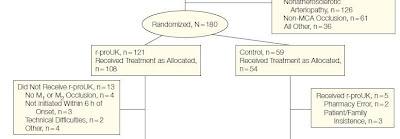
In this case, to strictly follow the ITT principle, the ITT analysis will include all 121 subjects in r-proUK group and all 59 subjects in Control group - purely based on the randomization, not based on whether or not the randomized subject receive the actual treatment or receive the wrong treatment. The ITT analysis was indeed used in the paper. However, since the PROACT II study was a proof of concept study, the analysis based on 'as treated' population should be used as well. 

With 'as treated' analysis, r-proUK group would have 121 subjects and Control group would have 54 subjects (see the comparison and the calculation below). 

The Number of Subjects for Analysis

	r-proUK	Control
As Randomized	121	59
As Treated	113 (121 randomized subjects - 13 subjects who did not receive treatment + 5 subjects who were randomized to Control group, but received r-proUK)	54 (59 randomized subjects – 5 subjects who were randomized to Control, but received r-proUK)

Typically, the safety analysis should always be based on the 'as treated' population since it really reflects the safety of patients under each treatment.

Fixed covariate, time dependent covariate, time varying covariate, and post-randomization covariate

A covariate is a variable that is possibly predictive of the outcome under study. A covariate may be of direct interest or it may be a confounding or interacting variable. Typically, when we use the term of ‘covariate’, we refer to the fixed covariate – a variable whose value will not change over the time. The fixed covariates include the demographic information (gender, age, race, …) and baseline characteristics (weight, height, baseline measure,…). Since ‘covariate’ typically means ‘fixed covariate’, we often drop the term ‘fixed’.

In contrary to the fixed covariate, time depedent covariate or time varying covariate (exact the same thing) refers to a covariate that is not necessarily constant through the whole study and has different values at different time points.  

There are many examples of the time dependent or time varying covariate in clinical trials or observational studies. For instance, if one wishes to examine the link between area of residence and cancer, this would be complicated by the fact that study subjects move from one area to another. The area of residency could then be introduced in the statistical model as a time-varying covariate.

When we analyze the CT lung densitometry data, we need to deal with the measurement of the lung volume – a reflection of the inspiration level. The CT densitometry measure is negatively correlated with the effort of the inspiration level. If we inhale more air into the lung, the lung density measure will be smaller and vice versa. In order for quantitative CT lung density to be valid endpoint, the corresponding measure of the lung volume (inspiration level) needs to considered and adjusted. If the outcome measure of CT lung density is measured at different times, there will also be corresponding measures of lung volumes at various times. The lung volume measure is considered as a time dependent covariate.

In clinical trials, the timing of the randomization is a critical point. The covariate can be separated into two groups: covariate measured or existed prior to the randomization and covariate measured after the randomization. The fixed covariates are measured or known prior to the randomization. The covariate measured after the randomization is called ‘post-randomization covariate’. The post-randomization covariate is usually also the time-dependent covariate.

When the time dependent covariate exists, we may be very tempted to include the covariate in the statistical analysis model. However, such approach could be biased if the time dependent covariate involves measures post-randomization.

A paper by Chen et al ‘A Note on Postrandomization Adjustment of Covariates” explained the issue:

“Examples include adjusting rescue therapies to explore the underlying difference of treatments which would have been observed in the absence of rescue medication, adjusting the level of patient compliance to estimate the treatment effect at the same compliance level, adjusting a postrandomization biomarker to evaluate the surrogating status of the biomarker to the clinical endpoint, and adjusting an intermediate endpoint or an endpoint other than the primary one to explore the therapeutic mechanism of one intervention.”

In its “ Guideline on adjustment for baseline covariates”, EMA explicitly opposes the use of adjustment for post-baseline covariates. In Section 4.2.5 (covariates affected by the treatment allocation), it states:

“A covariate that may be affected by the treatment allocation (for example, a covariate measured after randomisation such as duration of treatment, level of compliance or use of rescue medication) should not normally be included in the primary analysis of a confirmatory trial. When a covariate is affected by the treatment either through direct causation or through association with another factor, the adjustment may hide or exaggerate the treatment effect. It therefore makes the treatment effect difficult to interpret. However, such covariates (e.g. duration of treatment) might be included in secondary (exploratory) analyses and might offer the sponsor useful insights during the drug development process. Alternatively, subgroup analyses might offer similar insights.”

 The main concern for using the post-randomization covariates is the potential effect of treatment on the covariate measures. The covariates could become outcome measures or dependent variables instead of the independent variables. The post-randomization covariate measures may also be biased if there is inadequate blinding of the treatment allocation. In reality, it is not possible to defend that a post-randomization covariate is really a covariate and not impacted by the treatment. It is also difficult to confirm whether or not if the treatment effect of the experimental drug is mediated through the post-randomization or time-dependent covariates.

FDA does not have any guidance similar to EMA’s guidance on the use of post-randomization covariates. However, it is very rare to see the use of post-randomization covariates in the analysis of the primary efficacy endpoint in NDA or BLA submissions. There may be cases where post-randomization covariates are used in exploratory or ad-hoc analyses or used in analyses for non-randomized, observational studies.  

In sNDA ODAC Briefing document for Proscar, post hoc analysis was performed to include the post-randomization covariates. However, the briefing documents also commented “Adjustment for post-randomization variables (cores and volume) that are affected by treatment can introduce confounding bias and complicate causal interpretation.”

It has been noted that the time-dependent covaraites are more commonly used in survival analysis. See paper by Dr Lin “TIME-DEPENDENT COVARIATES IN THE COX PROPORTIONAL-HAZARDS REGRESSION MODEL”

Dealing with the time-dependent variable is a challenging statistical issue. The fundamental statistical problem is how to properly adjust for post-randomization variables, since, if the treatment has an effect on post-randomization variables, standard adjustment by regression modelling is susceptible to selection bias. The current proposal is to utilize Causal-Effects approach.  Dai et al had a pretty good introduction on this topic in their paper “Partially hidden Markov model for time-varying principal stratification in HIV prevention trials“. For details about the concept of Causal-Effects, the report of ”From Neurons to Neighborhoods: The Science of Early Childhood Development” by National Academy Press is a pretty good resource. 

Concept of "Person Year" in daily life

A while ago, I wrote a blog “Understanding person-year or patient-year”. While the concept of ‘person-year’ or ‘patient-year’ is mainly used in the epidemiology research (especially in the occupational health field) and clinical trials, the same concept may be used in the daily life.

This morning, I read an “Ask Marilyn” column on Parade.com. The question and answer applies the same concept of the ‘person-year’ or ‘patient-year’. With the concept of “person-year”, we need to combine the number of persons and the number of follow-up years in order to do the further calculation/statistical analyses. In the question/answer below, the number of family members and the number of days each family member stays need to be combined before the further calculation.

While 'person-year' may be more frequently used in the research field, the unit of time can be in years, months, days and they also can be called 'Person-time'. Person-time is an estimate of the actual time-at- risk in years, months, or days.

Question:

Nine family members will be renting a vacation property. The fee is $3,600 for 10 days. People will be staying for a varying number of days. I say the first step in figuring what each person owes is to divide the fee by nine. My husband says we should start by dividing the fee by 10—the number of days we have the rental. Who is right?

Marilyn responds:
Neither of you, but the dilemma is common. Here’s a way for anyone to solve this kind of vacation problem with any number of guests, days, etc. I’ll use your case as an example, and I’ll assume a family member who’s there surrounded by loved ones pays the same per day as one who gets the place all to him- or herself.

First, add up the number of days each family member stays. (Let’s say your nine people stay a total of 5+6+6+8+8+9+10+10+10 = 72 days.) Then divide the total rental fee by that figure ($3,600 ÷ 72 days = $50 per “person-day”). Each family member owes that result ($50) multiplied by the number of days he or she stays. So in this example, a person who stays five days owes $250. A person who stays all 10 owes $500.

Laboratory Tests: U.S. Conventional units versus SI units and Their Conversion Factors

In pretty much all clinical trials, laboratory tests are performed as a tool for diagnosing the disease, assessing the safety / tolerability, assessing the pharmacokinetics / pharmacodynamics and so on. A very common issue is the reporting units for laboratory tests. There are two different unit systems: conventional units and SI units.

U.S. Conventional Units (may also be referred as United States customary units): In the United States, most people express distances in inches, feet, yards, or miles. Those units, along with the units we use for speed, volume, and other quantities, are known as the U.S. Conventional System.

SI Units or Système Internationale: The International System of Units (abbreviated SI from French: Le Système international d'unités) is the modern form of the metric system and is the world's most widely used system of measurement, used in both everyday commerce and science. Most scientists and most countries now use SI units. SI units use the meter, the kilogram, the second, and the kelvin. Each base unit measures a different quantity. For example, the meter measures length, and the kilogram measures mass.

The units of these two systems are different, but the quantities they represent do not change. The units have a fixed relationship to each other. The laboratory results reported in U.S. Conventional Units can be converted into the results in SI Units or vice versa. The relationship to convert a value from one system to the other is called conversion factor. Below are some of the websites containing the conversion factors for common laboratory tests. The SI Conversion Calculator or conversion factor table provided by JAMA Author Instructions may be the most common one that has been used.

• SI Conversion Calculator
• Clinical Analyte Unit Conversion 
• SI Units for Clinical DataNormal Laboratory Values from AIDS.org
• AMA manual of style laboratory unit table 
• Conventional Units - International UnitsClinical Chemistry SI Conversion Factors 

Due to the differences between two unit systems, for a clinical trial where the central laboratory services are used, the decision needs to be made on which unit system is used for reporting the laboratory results to the investigators and to the sponsors. If it is a domestic trial in U.S., it is better to report the central laboratory test results in U.S. conventional units to the investigators. If it is multinational trial, it is better to report the central laboratory test results in S.I. units. For laboratory test results transferred to the sponsor, the results in both units can be requested.

The following may also be useful in understanding the different laboratory test units:

Factor Prefix Symbol for Lab Unit
10^12 tetra T
10^9 giga G
10^6 mega M
10^3 kilo k
10^(-3) milli m
10^(-6) micro µ
10^(-9) nano n
10^(-12) pico p
10^(-15) femto f
10^(-18) atto a

1 mL = 1 cc where mL is milliliter and cc stands for cubic centimeter
mg = milli gram = one-thousandth of a gram. 1 g = 1000 mg
1 mg = 1000 mcg or ug, here mc stands for "micro-" meaning "one millionth of".
In cell counts, the results may be reported as #/cumm, here cumm = mm^3 meaning per cubic millimeter.

For microbial measures (such as viral counts and viral loads), the log scale is commonly used. Microbial load (cfu/g or cfu/ml) can be expressed as log10. So, if you have 100,000 microbes that is 5 log, 10,000 microbes is 4 log, 1,000 is 3 log, 100 microbes is 2 log and 10 microbes is 1 log. Now, if you went from 100,000 microbes cfu/g to 10,000 microbes cfu/g that would be a 1 log reduction (5 - 4 log). If you went from 100,000 to 32,000 that would be a 0.5 log reduction (5 - 4.5 log) and so on.
If the microbial population went from 100,000 to 32,000 that would be a 0.5 log reduction (5 log - 4.5 log).
If the microbial population went from 100,000 to 320,000 that would be a 0.5 log increase (5.5 log - 5.0 log)

References:

Sunday, November 17, 2013